43 how to add data labels to a pie chart in excel on mac

How to show percentage in pie chart in Excel? - ExtendOffice Select the data you will create a pie chart based on, click Insert > I nsert Pie or Doughnut Chart > Pie. See screenshot: 2. Then a pie chart is created. Right click the pie chart and select Add Data Labels from the context menu. 3. Now the corresponding values are displayed in the pie slices. How to Create a Pie Chart in Excel - Smartsheet If want the category names to appear on or near the chart, right-click on the chart and click Add Data Labels …. By default, the numerical values are added. To add other labels, such as the categorical values or the percentage of the total that each category represents, right-click on the chart, then click Format Data Labels ….

Add column, bar, line, area, pie, donut, and radar charts ... Create a column, bar, line, area, pie, donut, or radar chart. Click in the toolbar, then click 2D, 3D, or Interactive. Click the left and right arrows to see more styles. Note: The stacked bar, column, and area charts show two or more data series stacked together. Click a chart or drag it to the sheet. If you add a 3D chart, you see at its center.

How to add data labels to a pie chart in excel on mac

Add or remove data labels in a chart - support.microsoft.com Click the data series or chart. To label one data point, after clicking the series, click that data point. In the upper right corner, next to the chart, click Add Chart Element > Data Labels. To change the location, click the arrow, and choose an option. If you want to show your data label inside a text bubble shape, click Data Callout. How to Add Data Labels to an Excel 2010 Chart - dummies Excel provides several options for the placement and formatting of data labels. Use the following steps to add data labels to series in a chart: Click anywhere on the chart that you want to modify. On the Chart Tools Layout tab, click the Data Labels button in the Labels group. A menu of data label placement options appears: None: The default ... How to format the data labels in Excel:Mac 2011 when ... Try clicking on Column or Row you want to set. Go to Format Menu Click cells Click on Currency Change number of places to 0 (zero) (if in accounting do the same thing. _________ Disclaimer: The questions, discussions, opinions, replies & answers I create, are solely mine and mine alone, and do not reflect upon my position as a Community Moderator.

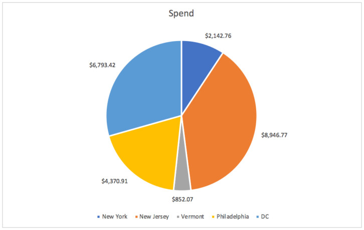
How to add data labels to a pie chart in excel on mac. A Step-By-Step Guide on How to Make a Pie Chart in Excel A pie chart provides a visual representation of data sets in an Excel worksheet. Pie charts help define data sets with values that add up to form a whole. The pie chart looks like a pie or a doughnut, representing the different data entries as a percentage of a total in proportional slices. Add a DATA LABEL to ONE POINT on a chart in Excel Method — add one data label to a chart line Steps shown in the video above:. Click on the chart line to add the data point to. All the data points will be highlighted.; Click again on the single point that you want to add a data label to.; Right-click and select 'Add data label' This is the key step! How to display leader lines in pie chart in Excel? To display leader lines in pie chart, you just need to check an option then drag the labels out. 1. Click at the chart, and right click to select Format Data Labels from context menu. 2. In the popping Format Data Labels dialog/pane, check Show Leader Lines in the Label Options section. See screenshot: 3. How to Make a PIE Chart in Excel (Easy Step-by-Step Guide) Related tutorial: How to Copy Chart (Graph) Format in Excel Formatting the Data Labels. Adding the data labels to a Pie chart is super easy. Right-click on any of the slices and then click on Add Data Labels. As soon as you do this. data labels would be added to each slice of the Pie chart.

Pie Chart in Excel | How to Create Pie Chart - EDUCBA Step 1: Do not select the data; rather, place a cursor outside the data and insert one PIE CHART. Go to the Insert tab and click on a PIE. Step 2: once you click on a 2-D Pie chart, it will insert the blank chart as shown in the below image. Step 3: Right-click on the chart and choose Select Data. How to Create Pie Charts in Excel (In Easy Steps) - Excel Easy 6. Create the pie chart (repeat steps 2-3). 7. Click the legend at the bottom and press Delete. 8. Select the pie chart. 9. Click the + button on the right side of the chart and click the check box next to Data Labels. 10. Click the paintbrush icon on the right side of the chart and change the color scheme of the pie chart. Result: 11. How to Insert Axis Labels In An Excel Chart | Excelchat We will go to Chart Design and select Add Chart Element Figure 6 - Insert axis labels in Excel In the drop-down menu, we will click on Axis Titles, and subsequently, select Primary vertical Figure 7 - Edit vertical axis labels in Excel Now, we can enter the name we want for the primary vertical axis label. Add a Data Callout Label to Charts in Excel 2013 In the upper right corner, next to your chart, click the Chart Elements button (plus sign), and then click Data Labels. A right pointing arrow will appear, click on this arrow to view the submenu. Select Data Callout. Once the Data Callout Labels have been added, you can re-position them by clicking on their borders and dragging to a new position.

How-to Add Label Leader Lines to an Excel Pie Chart - YouTube Step-by-Step Tutorial: how-to create label leader lines that connect pie labels that are outsi... How to add percentage to pie chart in excel - kasapwestcoast To add data labels, select the chart and then click on the + button in the top right corner of the pie chart and check the Data Labels button. Initially, the pie chart will not have any data labels in it. Select -> Insert -> Doughnut or Pie Chart -> 2-D Pie. Open Microsoft Excel and select the data that you want to create a pie. How Do You Add Text To Pie Chart In Excel For Mac - needtree To add data labels to a pie chart: How Do You Add Text To Pie Chart In Excel For Mac Free. Select the plot area of the pie chart. Right-click the chart. Select Add Data Labels. In this example, the sales for each cookie is added to the slices of the pie chart. How to Make a Pie Chart in Excel — Everything You Need to Know Right-click anywhere on pie-chart > Format Data Labels. 2. Label exists as simple numeric values (automatic). 3. Select desired label. Click Close. Editing Slices. 1. To edit slices in pie-chart, right-click anywhere on chart > Format Data Series. 2. To shift angle of a slice, set rotation angle by entering value or moving blue cursor. Click ...

32 Label Legend Google Sheets - Labels Information List

How to Create and Format a Pie Chart in Excel - Lifewire To add data labels to a pie chart: Select the plot area of the pie chart. Right-click the chart. Select Add Data Labels . Select Add Data Labels. In this example, the sales for each cookie is added to the slices of the pie chart. Change Colors

31 How To Label Vertical Axis In Excel

Add Data Labels to an Excel Pie Chart - Home and Learn The chart is selected when you can see all those blue circles surrounding it. Now right click the chart. You should get the following menu: From the menu, select Add Data Labels. New data labels will then appear on your chart: The values are in percentages in Excel 2007, however. To change this, right click your chart again.

33 How To Label Axis On Excel Mac 2016 - Labels For Your Ideas

Change the look of chart text and labels in Numbers on Mac If you can't edit a chart, you may need to unlock it. Change the font, style, and size of chart text Edit the chart title Add and modify chart value labels Add and modify pie chart wedge labels or donut chart segment labels Modify axis labels Edit pivot chart data labels Note: Axis options may be different for scatter and bubble charts.

31 What Is A Category Label In Excel - Labels Database 2020

Excel charts: add title, customize chart axis, legend and ... To add a label to one data point, click that data point after selecting the series. Click the Chart Elements button, and select the Data Labels option. For example, this is how we can add labels to one of the data series in our Excel chart: For specific chart types, such as pie chart, you can also choose the labels location.

Format data labels in a chart in Office 2016 for Mac - Office Support

How to Make a Pie Chart in Excel: 10 Steps (with Pictures) Add your data to the chart. You'll place prospective pie chart sections' labels in the A column and those sections' values in the B column. For the budget example above, you might write "Car Expenses" in A2 and then put "$1000" in B2. The pie chart template will automatically determine percentages for you.

34 What Is A Data Label - Labels Design Ideas 2020

Office: Display Data Labels in a Pie Chart 2. If you have not inserted a chart yet, go to the Insert tab on the ribbon, and click the Chart option. 3. In the Chart window, choose the Pie chart option from the list on the left. Next, choose the type of pie chart you want on the right side. 4. Once the chart is inserted into the document, you will notice that there are no data labels.

Excel chart elements not showing Mac, mac office 365 excel 2021 chart format

Create a chart in Excel for Mac - support.microsoft.com Click a specific chart type and select the style you want. With the chart selected, click the Chart Design tab to do any of the following: Click Add Chart Element to modify details like the title, labels, and the legend. Click Quick Layout to choose from predefined sets of chart elements.

How to Make a Pie Chart in Excel: 10 Steps (with Pictures)

How to Use Cell Values for Excel Chart Labels - How-To Geek Select the chart, choose the "Chart Elements" option, click the "Data Labels" arrow, and then "More Options.". Uncheck the "Value" box and check the "Value From Cells" box. Select cells C2:C6 to use for the data label range and then click the "OK" button. The values from these cells are now used for the chart data labels.

Share :